Python Tutorial Part 3: Libraries for Data Analysis and Machine Learning
Part 3: Machine Learning Libraries of this compact Python tutorial introduces frequently used libraries for data analysis and Machine Learning. The packages NumPy, Matplotlib and Pandas used for data analysis and visualization are discussed first. Next, the Machine Learning library Scikit-Learn is explained using as example a failure prediction task. Finally, the packages Keras and Tensorflow are explained and used to create and train an artificial neural network for image recognition.
Motivation
Machine Learning is a branch of Artificial Intelligence that enables systems to automatically learn new information based on training data, rewards, or other rules. Machine Learning applications such as image processing or failure prediction are often developed with Python.
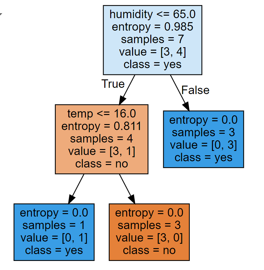 Python has freely available libraries that cover all relevant Machine Learning algorithms:
classification, regression, decision tree methods, cluster analysis, artificial neural networks.
The usual steps of the Machine Learning pipeline, such as data preparation, model selection, training,
validatation and finally prediction, are implemented using a set of matching libraries.
1 Python libraries for data analysis
| Top |
Frequently used Python libraries for data analysis are:
- NumPy - provides support for creating and manipulating multidimensional arrays and random numbers
- Matplotlib - provides functions for data visualization
- Pandas - provides special data structures and methods for processing tabular data, e.g. Series, DataFrames
The following sections give a short description for each package and illustrate its basic usage with a representative code fragment.
| Top |
1-1 NumPy
NumPy is a Python library for data management, providing support for array creation and manipulation. NumPy arrays have a fixed size, contain elements of the same data type and efficiently support elementwise operations. With NumPy, you can create arrays, initialize and extract data, perform elementwise operations on arrays, sort, search, count elements and calculate array statistics.
NumPy 1D and 2D-Arrays
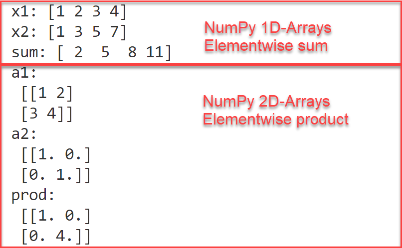
This example shows the creation of 1D and 2D arrays. First, two 1D-arrays x1 and x2 are created, each with four elements: x1 from a list using the array constructor np.array(), x2 as a number sequence (start: 1, end: 8, step size 2) using the function arange(). The expression sum = x1 + x2 calculates the element-wise sum of the two NumPy arrays. Alternatively, the element-wise sum of two NumPy arrays can also be calculated with sum = np.add(x1, x2). Next, two 2D-arrays a1 and a2 are created: a 2x2 matrix a1 with elements 1, 2, 3, 4, and a2 as a 2x2 identity matrix using the eye() function. Finally, the element-wise product is calculated for the two 2D arrays using prod = a1 * a2.
Python-Code: Use NumPy Arrays
Functions used: array, arange, eye
import numpy as np# One-dimensional NumPy arraysx1 = np.array([1, 2, 3, 4])x2 = np.arange(1, 8, 2)sum = x1 + x2 # Elementwise sumprint('x1:', x1, '\nx2:', x2, '\nsum:', sum)# Two-dimensional NumPy arraysa1 = np.array([[1, 2], [3, 4]], )a2 = np.eye((2))prod = a1 * a2 # Elementwise productprint('a1:\n', a1, '\na2:\n', a2, '\nprod:\n', prod)
NumPy nd-Arrays
NumPy supports the creation of general n-dimensional arrays through the initialization functions zeros, eye,and random as in:
# NumPy ndarray with 3 dimensions
x = np.zeros((2, 3, 2))
# NumPy ndarray with 4 dimensions
x = np.eye((2, 3, 2, 4))
# NumPy ndarray with 5 dimensions
x = np.random((2, 3, 4, 5))
These higher-dimension arrays are frequently needed to store data for Machine Learning algorithms.
NumPy arrays vs. Python lists
What is the difference between NumPy arrays and Python's built-in lists, which is to be used in which context? Python lists are of variable length, may contains elements of mixed data type and support a reduced set of operations as needed to store and retrieve data efficiently. NumPy arrays have fixed size, contain elements of the same data type, and efficiently support element-wise operations and a variety of statistical functions. They are therefore preferably used in data analysis tasks, where you need all these element-wise operations and statistical functions.
Adding NumPy arrays vs. Python lists
The following example shows the difference in using the "+" operator on Python lists vs. NumPy arrays.
➔ If you add two Python lists, the result is a new list that contains the elements of both lists.
➔ If you add two NumPy arrays, the result is a new array whose elements are formed by elementwise
addition. Element-wise addition can also be done with Python lists, then a loop or the so-called list comprehension must be used.
import numpy as np# Create 2 Python listslist1 = [1, 2, 3, 4]list2 = [5, 6, 7, 8]# Convert them to NumPy arraysarr1 = np.array(list1) # NumPy Array [1 2 3 4]arr2 = np.array(list2) # NumPy Array [5 6 7 8]# Adding Python lists means: appendingsum = list1 + list2print(sum) # [1, 2, 3, 4, 5, 6, 7, 8]# Adding NumPy arrays means: elementwise additionsum = arr1 + arr2print(sum) # [6 8 10 12]
| Top |
1-2 Matplotlib
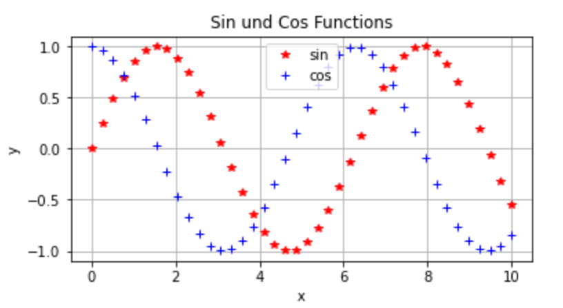
Matplotlib is a Python library for data visualization that supports the creation of various types of charts via the pyplot package: line, scatter, histograms, bar charts, one- and two-dimensional plots, static or interactive. Frequently used commands are plot for one-dimensional and surf for two-dimensional plots. The plot command receives as parameters the x and y coordinates of the data to be plotted, and optionally a string with formatting information. There are also many options for adding labels, titles, legends, etc.
Create a line plot with Matplotlib
Functions: figure, plot, title, grid, legend, xlabel, ylabel
import numpy as npimport matplotlib.pyplot as pltx = np.linspace(0,10,40) # x-valuesy1 = np.sin(x);y2 = np.cos(x); # y-valuesfig = plt.figure(figsize=[6, 3])plt.plot(x, y1,'r*', label='sin');plt.plot(x, y2,'b+', label='cos');plt.title('Sin and Cos Functions');plt.grid(True)plt.legend(loc="upper center")plt.xlabel('x');plt.ylabel('y');
Create a histogram with Matplotlib
Functions: hist, show
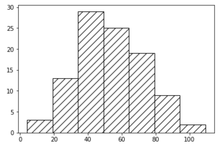
A histogram is the graphic representation of the frequency distribution of a variable. The data of the variable are sorted according to their size and divided into a number of classes or bins that can, but do not have to be, of the same width.
import matplotlib.pyplot as pltimport numpy as np# Create 100 random numbers# with mean 50 and standard deviation 20x = np.random.normal(50, 20, 100)# Create histogram with 7 binsplt.hist(x, 7, density=False, fill=False, hatch='//')plt.show()
| Top |
1-3 Pandas
Pandas is a Python library for creating and manipulating spreadsheet-like data. Pandas provides support for loading large data files (csv, xls) into the program's memory and then further cleanse and visualize the data. Pandas functions such as iloc(), loc(), resample() are used to select rows/columns/cells, to group and aggregate data etc.
Pandas vs Python Lists and NumPy Arrays
Pandas is suitable for loading an entire already existing dataset into a DataFrame.
Although it is possible to create an empty DataFrame with given column names and then growing
it by appending rows, this is not the intended use case and has a bad performance.
Pandas is meant to be used together with Python lists and NumPy arrays.
So first create Python lists for the columns that you need to store, here you can use append and it is fast.
Then create a dictionary, that associates to each columns name its values, and finally create
a Pandas DataFrame from this dictionary - as in our example.
There are a number of functions that support conversion between Pandas DataFrame columns and Python lists,
such as tolist().
| Top |
Read from and write to files using Pandas
Functions: read_excel, to_csv
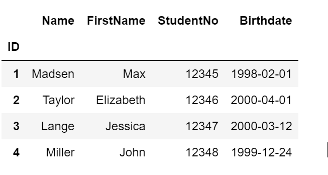
In this example we read the data stored in the excel sheet students.xlsx, store them in a DataFrame df and then write them to a csv-file.
import pandas as pd# Read data from students.xlsxdf = pd.read_excel('students.xlsx', index_col=0)# Write data to a csv filedf.to_csv('students.csv', index=True, sep = ';')df
Create and plot Pandas DataFrame
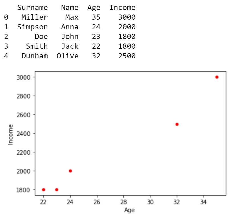
import pandas as pdpersons = {"Surname": ["Miller", "Simpson", "Doe", "Smith", "Dunham"],"Name": ["Max", "Anna", "John", "Jack", "Olive"],"Age": [35, 24, 23, 22, 32],"Income": [3000, 2000, 1800, 1800, 2500]}# Create data frame from dictionarydf = pd.DataFrame(persons)print(df)# Scatter-plot Income vs Agedf.plot.scatter(x = 'Age', y = 'Income', c='Red');
2 Python libraries for Machine Learning
Machine Learning algorithms are supported in Python by the Scikit-Learn package. For implementing Deep Learning, i.e. powerful artificial neural networks, Python offers several program libraries, including PyTorch, JAX, Tensorflow and Keras. These packages provide similar functionality for building and using deep learning models. PyTorch, JAX and Tensorflow differ in the internal implementation of the procedures and also in the use of the API functions. Keras is a package with wrapper functionality that can be used as a backend with any of the three other packages.
| Top |
2-1 Scikit-Learn
Scikit-Learn is a Python library for Machine Learning that provides support for the usual steps of supervised and unsupervised learning: data preparation, training and model evaluation, as well as powerful algorithms for classification, regression and clustering problems. Scikit-Learn is used together with NumPy, Matplotlib and Pandas: with Pandas, we read data from files and convert them to NumPy arrays, with Matplotlib, we plot them, with NumPy, we pass data as arguments to Scikit-Learn functions.
Scikit-Learn algorithms are summarized under the general term estimator. An estimator is an object that provides functions for building models, in particular a fit method that trains the model on given data. Estimators are divided into classifiers, regressors and clusterers, each according to the Machine Learning category to which they belong. The UML class diagram below shows an excerpt from the Scikit-Learn class hierarchy, with the dependencies, attributes and methods of the estimators DecisionTreeClassifier, RandomForestClassifier, DecisionRegressor, RandomForestRegressor, KMeans and AgglomerativeClustering. From the diagram it can be seen that all estimators are derived from the BaseEstimator class, inheriting its fit method, and also have uniformly named methods such as predict() and score(), as well as parameters that configure the structure of the model.
Install Scikit-Learn
Scikit-Learn is installed via pip using its full name:
pip install scikit-learn
Example
Failure classification using DecisionTreeClassifier
In this example we show how to train a decision tree model with Scikit-Learn and subsequently use it for the classification of failures. We have a small labelled data-set containing measurements, some observations have led to a device failure. The question to be answered is: what combination of measurements leads to a failure?
Data set data.csv
The data set data.csv contains 8 measurements of temperature and humidity, and a column "failure" that contains the label of one measurement. The first row contains the column headers. First row can be interpreted as follows: for temperature 20.3 degrees (Celsius) and humidity 60%, there has been no failure.
id;temp;humidity;failure
1;20.3;60;no
2;35.6;80;yes
3;40;55;yes
4;25;50;no
5;17;60;no
6;15;75;yes
7;20.3;80;yes
8;35.6;60;yes
Step 1: Read data from file
First step is to read the data from the file using Pandas' read_csv() function. This function takes a number of parameters that control the reading process, we specify here: file: the name of the file, header=0: row with index 0 contains the column headers, index_col = 0: column with index 0 contains the row headers.
import pandas as pd# 1.file = "https://evamariakiss.de/tutorial/python/data2.csv"df = pd.read_csv(file, header=0, sep = ";", index_col=0)print('DataFrame:\n', df);
Step 2: Extract features and target variable
Next we extract features and target variable in NumPy arrays x and y. This must be done since the Scikit-Learn Classifier and more precisely the fit-method expects NumPy arrays as parameters.
# 2.x = df.iloc[:,0:2].to_numpy() # Extract featuresy = df[['failure']] # Extract target variabley = y.values
Step 3: Create a train-test-split
In Step 3 we split the data set into training and validation data using Scikit-Learn's train_test_split. The parameter test_size specifies that 0.1 of the data set is used for testing / validation.
from sklearn import model_selection as ms# 3.X_train, X_test, y_train, y_test = \ms.train_test_split(x, y, test_size=0.1, random_state=1)
Step 4: Train a decision tree
In Step 4 we create a new instance of the DecisionTreeClassifier, conveniently named "model". We train this model using the fit function and training data have been created previously using the train_test_split-function.
from sklearn import tree, model_selection as ms# 4.model = tree.DecisionTreeClassifier(criterion='entropy', splitter='best')model.fit(X_train, y_train) # Train decision tree
Step 5: Visualize the decision tree
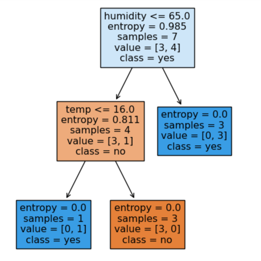
We visualize the decision tree using ScikitLearn's visualization functions plot_tree or alternatively export_graphviz. Both functions create a decision tree visualization that specifies for each node the splitting criteria, the entropy, the number of samples in that node and how many samples are in each class. While plot_tree is simpler, export_graphviz produces a sharp graph in SVG-format, suitable for re-use in websites and presentations.
Visualization using plot_tree
import matplotlib.pyplot as pltfrom sklearn import tree# 5. Visualize decision treefig, ax = plt.subplots(figsize=(5, 6))tree.plot_tree(model, filled=True,feature_names=df.columns[0:2],class_names=['no','yes'])plt.show()
Visualization using export_graphviz
import graphviz as gvimport IPython.display as dispfrom sklearn.tree import export_graphviz# 5. Visualize decision treedot=export_graphviz(model, out_file=None,filled=True,feature_names=df.columns[0:2],class_names=['no','yes']);graph = gv.Source(dot)style = ''display(disp.HTML(style))display(graph)

Steps 1 to 5: the complete code
Finally, we put together the code from steps 1 to 5 in one single script.
import pandas as pdimport matplotlib.pyplot as pltfrom sklearn import tree, model_selection as ms# 1.file = "https://evamariakiss.de/tutorial/python/data2.csv"df = pd.read_csv(file, header=0, sep = ";", index_col=0)print('DataFrame:\n', df);# 2.x = df.iloc[:,0:2].to_numpy() # Extract featuresy = df[['failure']] # Extract target variabley = y.values# 3.X_train, X_test, y_train, y_test = \ms.train_test_split(x, y, test_size=0.1, random_state=1)# 4.model = tree.DecisionTreeClassifier(criterion='entropy', splitter='best')model.fit(X_train, y_train) # Train decision tree# 5.fig, ax = plt.subplots(figsize=(5, 6)) # Visualize decision treetree.plot_tree(model, filled=True, feature_names=df.columns[0:2], class_names=['no','yes'])plt.show()
| Top |
2-2 Keras
Keras is a Python package used as a user-friendly programming interface for various Machine Learning frameworks such as Tensorflow, PyTorch and JAX.
Keras provides two classes for creating a neural network: Sequential and Functional, both of which support creating multi-layer networks. The Sequential API allows layers to be assembled sequentially, while the Functional API can be used to create more complex arrangements of layers.
The layers of an artificial neural network are implemented in Keras by the classes of the layer API, that has layers such as Conv2D, MaxPooling2D, Flatten, Dense, LSTM etc. Each layer class has a weight matrix, a size specification for the number of neurons used (units), a format description the input data (input_shape), an activation function (activation), and a number of other parameters that control the shape of the layer.
The usual steps in creating a neural network (create model, train model, validate and use model) are carried out in Keras using the functions compile(), fit() and predict().
| Top |
2-3 Tensorflow
Tensorflow is a framework for Machine Learning that is particularly used for applications in image and speech recognition.
Tensorflow offers programming interfaces for various programming languages, especially Python, Java and C++, of which the most used and stable interface is the Python API. The Tensorflow API documentation is extensive and the examples provided can be practically followed by running the linked Colab notebooks.
Tensorflow will initially be used for tasks in image and video processing, both for image recognition (is there an object?) and image classification (what object is it?). Training a model in image classification is very complex - here you can use Tensorflow to access pre-trained models and simply use them for classification.
What exactly is a tensor? In Machine Learning parlance, a tensor is a multidimensional constant data structure with its own set of operations, which represents the mathematical unit of an artificial neural network. In contrast to the well-known multidimensional data structures such as lists or matrices, a tensor can not only have several dimensions, but also several axes.
https://www.tensorflow.org/guide/tensorimport tensorflow as tfimport numpy as nprank_3_tensor = tf.constant([[[0, 1, 2, 3, 4],[5, 6, 7, 8, 9]],[[10, 11, 12, 13, 14],[15, 16, 17, 18, 19]],[[20, 21, 22, 23, 24],[25, 26, 27, 28, 29]],])print(rank_3_tensor)
| Top |
Install Keras and Tensorflow
The installation of Keras requires to install it together with a backend, e.g. Tensorflow,
PyTorch or JAX.
The recommended way is to create a dedicated environment using conda, use the last version of pip,
and check the installation notes in advance.
Steps for installing the current version Keras 3.5 with Tensorflow 2.16:
conda create conda-dl
conda activate conda-dl
pip install --upgrade keras==3.5.0
pip install tensorflow==2.16.2
When using Anaconda for package and environment management, the packages will be
installed in
| Top |
2-4 Image classification with Keras and Tensorflow
This example shows how an artificial neural network for digit classification is trained using Keras / Tensorflow and used for prediction on new self-created images. The goal is to create and train a model that can correctly classify handwritten digits (gray-white images in 28x28 pixel format representing the digits 0,1,2,...,9).

The example is based on the Simple MNIST convnet demo from the collection of Keras code examples. The complete source code with additional explanations is available online as a Google Colab Notebook.
Step 1: Read and prepare data
The MNIST digit dataset consists of 60,000 hand-written images representing the digits 0, 1, 2, ..., 9 as
28x28 pixels and can be loaded directly via the Keras-package mnist.
This dataset is used as the training and validation data set.
In a first step, the data used for training must be loaded from their storage place and prepared,
so that they can be used as input for the algorithm.
Data preparation means that image data must be converted into a given numerical form, normalized and encoded.
Functions used: load_data(), reshape(), to_categorical().
In the next code blocks we use the standalone Keras package.
An alternative would be to use the Keras package that ships with Tensorflow.
In this case, you would have to write
from tensorflow.keras.datasets import mnist instead of
from keras.datasets import mnist.
Python code: Data preparation with Keras
import numpy as npimport matplotlib.pyplot as pltfrom keras.datasets import mnistfrom keras.utils import to_categoricalprint("1. Load MNIST dataset")(trainX, trainY), (testX, testY) = mnist.load_data()# Display dimensions of train and test dataprint('Train: X=%s, Y=%s' % (trainX.shape, trainY.shape))print('Test: X=%s, Y=%s' % (testX.shape, testY.shape))print("2. Prepare data")trainX = trainX.reshape((trainX.shape[0], 28, 28, 1))testX = testX.reshape((testX.shape[0], 28, 28, 1))# Normalize data to [0, 1]trainX = trainX.astype("float32") / 255.0testX = testX.astype("float32") / 255.0# Target variable is coded as categorical datatrainY = to_categorical(trainY)testY = to_categorical(testY)print('Train: X=%s, Y=%s' % (trainX.shape, trainY.shape))print('Test: X=%s, Y=%s' % (testX.shape, testY.shape))
Output: Data preparation with Keras

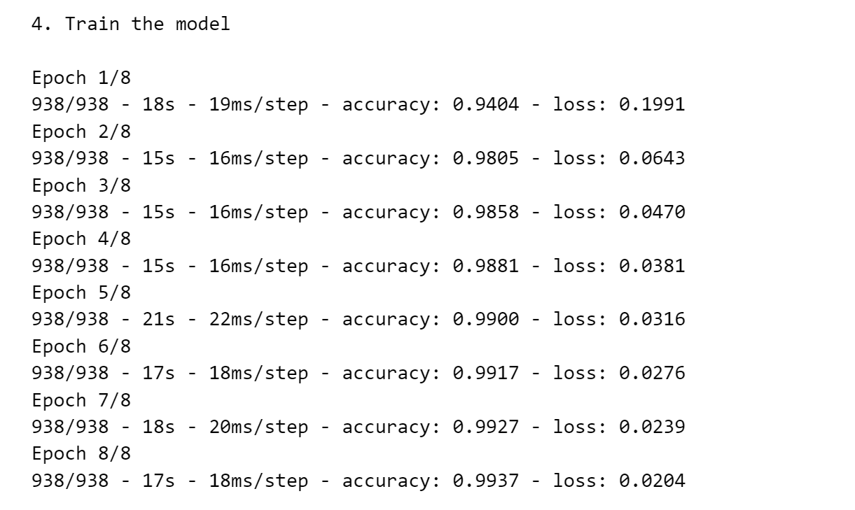
Step 2: Define and train model
In this step, a deep learning model is created, configured for the training phase, and then trained using
the training data prepared in Step 1.
A new sequential model is created by adding layers as needed: a Conv2D-layer that detects the image,
followed by a MaxPooling2D-layer that condenses the image, reducing large areas containing only 0's
that would unnecessarily increase the size of the model.
An activation function can be specified for each layer.
Classes used: Sequential, Conv2D, MaxPooling2D, Flatten, Dense
Methods used: compile(), summary(), fit(), save()
Output# Define the modelfrom keras.models import Sequentialfrom keras.layers import Conv2D, MaxPooling2D, Dense, Flattenprint("3. Define the model")model = Sequential()model.add(Conv2D(32, (3, 3), activation='relu', input_shape=(28, 28, 1)))model.add(MaxPooling2D((2, 2)))model.add(Conv2D(64, (3, 3), activation='relu'))model.add(MaxPooling2D((2, 2)))model.add(Flatten())model.add(Dense(10, activation='softmax'))model.compile(loss='categorical_crossentropy', metrics=['accuracy'])model.summary()# Train the modelprint("4. Train the model\n")model.fit(trainX, trainY, epochs=8, batch_size=64, verbose=2)# Save the modelmodel.save('digits_model.keras')
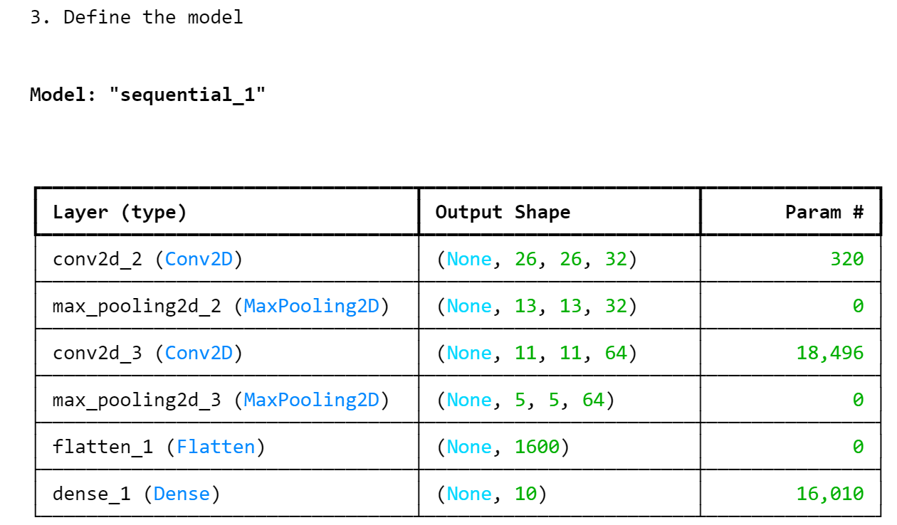
import tensorflow as tfinput_shape = (28, 28, 1) # Input shape for 28x28 grayscale imageinput = tf.keras.Input(shape=input_shape) # Input tensoroutput = tf.keras.layers.Conv2D(filters=32, kernel_size=(3,3), activation='relu')(input)print(output.shape)
Step 3: Evaluate the model
In this step, the quality of the model is determined using the indicators loss and accuracy (trust probability).
The loss parameter was used to configure which performance metric should be minimized during training.
The confidence probability is the probability that a correct prediction will be made for an observation.
Functions used: evaluate()
print("5. Evaluate the model\n")score = model.evaluate(testX, testY, verbose=0)print("Test loss:", score[0]) # Output: Test loss: 0.03print("Test accuracy:", score[1]) # Output: Test accuracy: 0.99
Step 4: Use the model for classification
This step uses the previously created model to correctly classify new images.
4-1 Load image
First, the image to be classified must be loaded and encoded.
Specifically, an image representing the number 5 is loaded either from the file system or from an URL
and converted into the numerical representation required by the model.
The self-defined function encode_image()
loads an image passed as filename and returns a numerical representation of the image.
Functions used: load_img(), img_to_array()
from keras.preprocessing.image import load_img, img_to_arrayfrom keras.utils import get_filefrom keras.models import load_modelimport numpy as npdef encode_image(filename):img = load_img(filename, color_mode = 'grayscale', target_size=(28, 28))img = img_to_array(img)img = img.reshape(1, 28, 28, 1)img = img.astype('float32') / 255.0return img
4-2 Load model and perform prediction
Next, the image is encoded using the previously tested function encode_image().
Then the model is loaded from the previously saved *.keras file,
and the prediction on the encoded image is carried out using the predict()-method.
The classification using the predict function in line 9 returns
a NumPy array "digit" of 9 integer values as a result,
where a 1 in position i means that the image was classified as a number i.
The method keras.utils.get_file() downloads a file from a URL.
The method keras.models.load_model() loads a model that has been previosly saved as file.
The method predict() returns predictions for the input samples.
# Load and encode the image: digit-2, digit-5 or digit-7img_url = 'https://evamariakiss.de/tutorial/python/images/digit-2.png'img = Nonetry:file = get_file(origin=img_url)img = encode_image(file)model = load_model('digits_model.keras')digit = (model.predict(x=img, verbose="auto") > 0.5).astype("int32")print(digit[0])print("The image represents the number:")print(list(digit[0]).index(1)) # Output: The image represents the number: 2except Exception as error:print("Error: %s" % error)
References and tools
- [1] Python Documentation at python.org: docs.python.org/3/tutorial/
- [2] Anaconda: anaconda.com/: package management system, also needed for installing Jupyter Notebook
- [3] PIP Packet Manager: pypi.org/project/pip/
- [4] Conda Cheatsheet: conda-cheatsheet.pdf
- [5] Visual Studio Code: code.visualstudio.com/
- [6] NumPy: numpy.org/ – Arrays, Random Number Creation
- [7] Matplotlib: matplotlib.org/ – Data Visualization, Plotting
- [8] Pandas: pandas.pydata.org/ – DataFrames, Series
- [9] Scikit-Learn: scikit-learn.org – Algorithms for Machine Learning